Section 20.2 Estimating the Time Constant
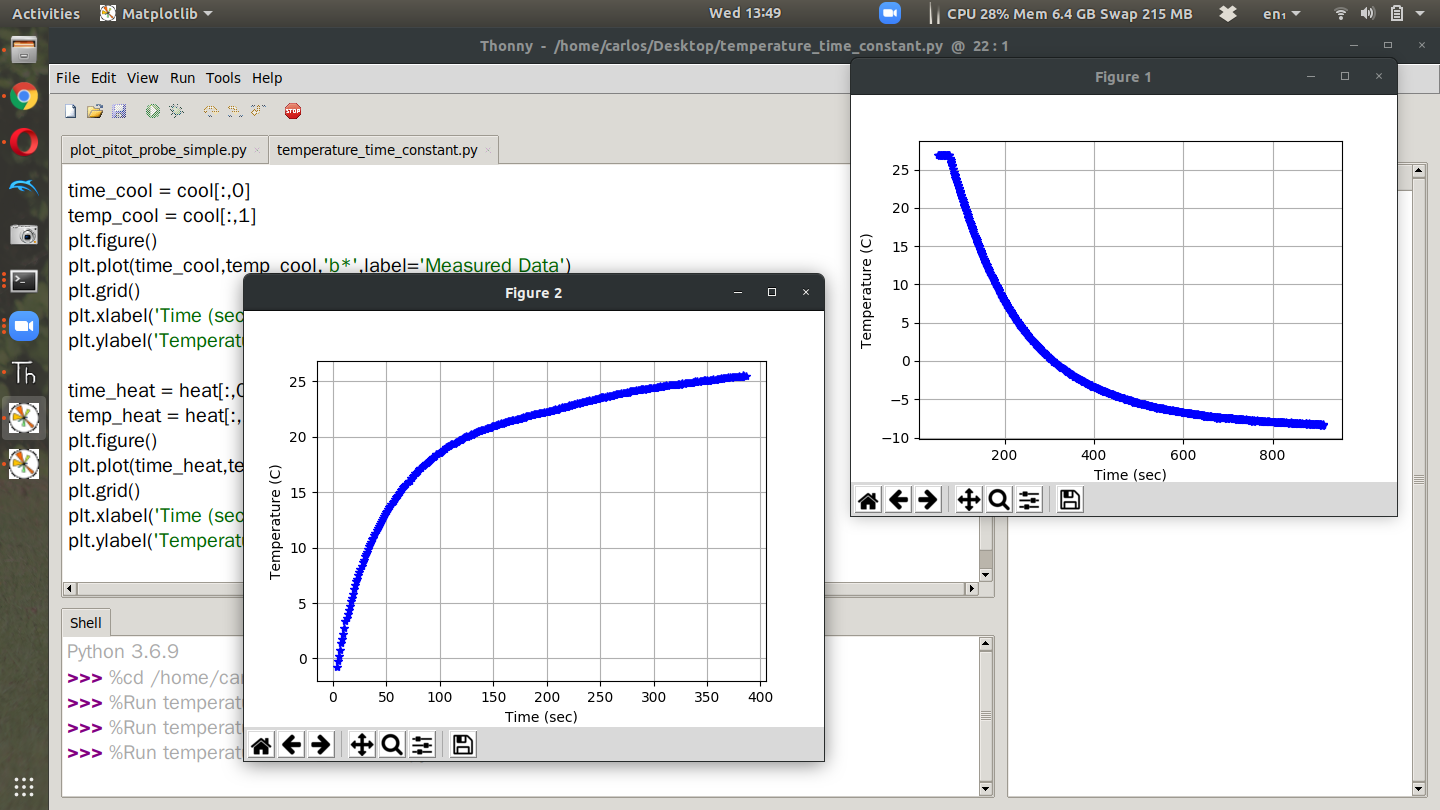
I did the first two examples (using a fridge) and plotted both data sets in the same script as shown below. I opted to use method 1 (see chapter 9) from the datalogging project and just have the data print to Serial and then unplug the CPX when I’m done taking data and copy and paste the data into a text file.
At this point it’s possible to get the time constant by remembering that the settling time (time it takes the temperature to settle out) is equal to 4 times the time constant (\(\tau\)) and thus the time constant is the settling time divided by 4. After computing the settling time for both data sets and overlaying the equations on the measured data I get these two plots.
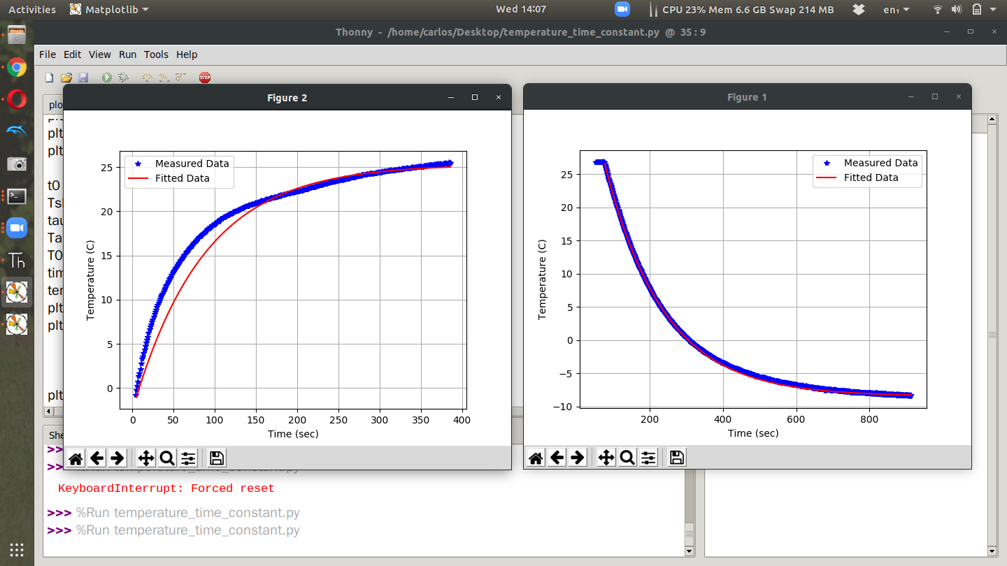
What was interesting was that the time constant for heating up was 62.5 seconds and for cooling down it was 155 seconds. The time to get cold was way slower than heating up. I’m not a heat transfer expert so I won’t comment as to why this happened. One other import note I’d like to mention is the cool down phase was much more accurate than the heat up phase. This is most likely because when I pulled the thermistor out of the fridge I touched it with my hands and then moved it to a table. There was also alot more airflow outside the fridge which would change the overall dynamics. Still, the fitted data matches up pretty well and I hope yours does too.
