Section 18.2 Statistics of your Data
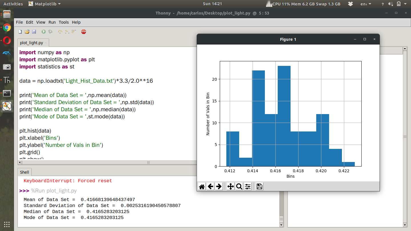
If you allow the light source to be constant you’ll notice that the data is quite noisy. What I’d like you to do for part 2 of this lab is take 1000 data points with the photocell with as constant of a light source as possible. Do this for three different light ranges. Low Light, ambient light and then sunlight if you’re outside. If you’re completing this assignment late you can use a flashlight as your third light source. With the three different data streams, create a histogram of the data with appropriate labels and compute the mean, median, and standard deviation of the data stream. Here is my example code showing code to get mean, median, and standard deviation as well as create the histogram. Notice in my code I imported the statistics module to compute the mode. Although it worked in my code, it’s not typical to compute the mode of a continuous variable because often times you will not ever get the same value twice. Still, feel free to compute the mode if you so desire.
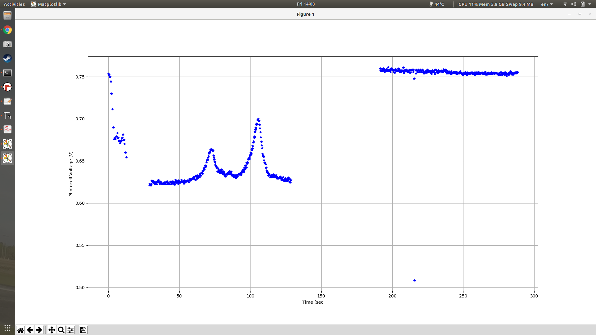
Again make sure to convert to voltage and then Lux before you plot that way you can see what the noise level is in volts and Lux. When I ran this experiment for a second time my CPX started and stopped 3 separate times. You’ll see in the time series plot below that the voltage dipped in the first set and the second data set had some weird bumps probably from me changing tabs on my chrome tab. The photocell was close to my computer so that effected it. Thankfully the 3rd data set looked pretty good.
The only problem with the 3rd data set is that I put my hand over it for testing purposes. Because of that I had to remove those outliers. To do that I computed the current mean and standard deviation and then threw out all data points that were 3 standard deviations away from the mean. The code looks like this.
##COMPUTE CURRENT MEAN AND DEV

mean = np.mean(voltage)

dev = np.std(voltage)

print(mean,dev)

time = time[voltage > mean - 3*dev]

voltage = voltage[voltage > mean - 3*dev]

time = time[voltage < mean + 3*dev]

voltage = voltage[voltage < mean + 3*dev]

###COMPUTE NEW MEAN,STD

mean = np.mean(voltage)

dev = np.std(voltage) print(mean,dev)
Once I did all that clean up I was able to get a nice time series plot of my data.
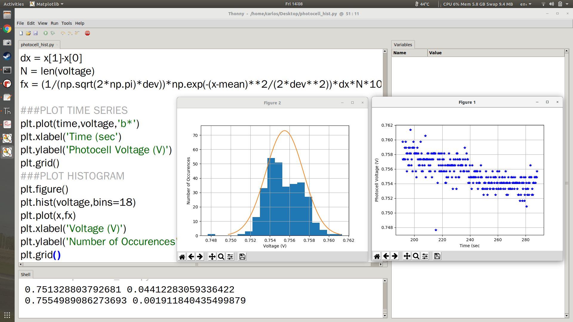
I also was able to plot the Normal Gaussian Distribution on top of the histogram. You can see that in the left plot in orange. The code to do that is shown below where the 72 in the plot is the "height" of the histogram. Note that your histogram will have a different height and you will need to get that specifically from your plot.
###COMPUTE THE NORMAL DISTRIBUTION

x = np.linspace(-3*s+mu,3*s+mu,100)

pdf = 1.0/(s*np.sqrt(2*np.pi))*np.exp((-(x-mu)**2)/(2.0*s**2)) * (s*np.sqrt(2*np.pi)) * 72
The equations above make a time series from +-3 standard deviations from the mean and then plot the PDF of a normal Gaussian distribution. The only extra thing you have to do is multiply by (s*np.sqrt(2*np.pi)) * 72 which first causes the height of the PDF to be 1 and then multiply by 72 which again is the height of the histogram which will be different for your system.
