Section 21.2 Estimating Parameters
After trimming the data and removing some bias it was time to get my damping constant and damped natural frequency. There are a few equations that can help you obtain these parameters. First, the settling time is the length of time it takes for the oscillations to settle. The settling time can be used to find the damping constant. This is equal to:
\begin{equation}
\sigma = \frac{4}{T_s}\tag{21.2.1}
\end{equation}
For my data set the settling time was about 1.25 seconds which gave a damping constant of 3.2. Once I had the damping constant I could obtain the damped natural frequency. This was done by measuring the distance between two peaks in the data set. There is a peak at around 0.5 seconds and another at around 0.95 seconds. I can use this to compute a period T. Period can be computed to angular frequency using the equation below.
\begin{equation}
\omega_d = \frac{2\pi}{T}\tag{21.2.2}
\end{equation}
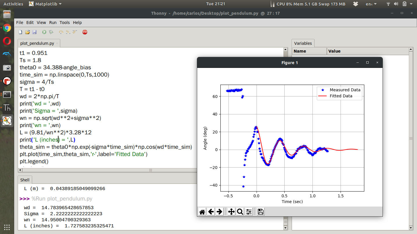
Using the period in my wave form I obtained a damped natural frequency of about 14.8 rad/s. Using these values I can plot the simulated data on top of the measured data noting that my initial angle was about 35 degrees minus the bias of 8 degrees. When I first plotted the data I noticed that my fit wasn’t entirely perfect. My period was correct but my damping rate was too high. I realized it was because my settling time was too big. I increased the settling time to 1.8 seconds and got this plot here. You can see that my fitted data lined up almost perfectly with my measured data.