Section 19.3 Feedback Control
Feedback control can be its own course or multiple courses but can be broken down into a few simple steps. The goal of feedback control is to drive the “state” of a “system” to a desired “command” by sending a “control” signal to the “system”. The figure below shows a standard block diagram for a dynamic system.
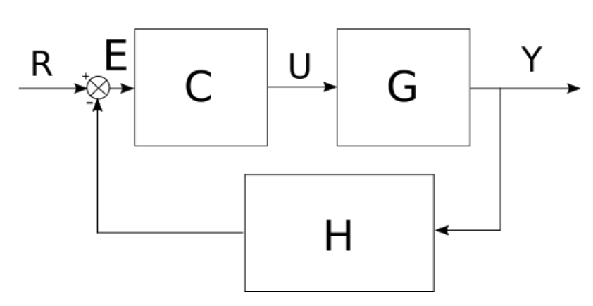
In this figure, R is the reference signal or the commanded signal. The reference signal feeds into a summation block where the reference signal is substracted from the measured signal. The measured signal is the output of the H block which represents the sensor. The output of the summation block is the error signal E. The error signal feeds into the controller C and outputs the control signal U to the plant system G. The output of the plant G is Y or the state. The state Y feeds into the sensor block H to measure this signal and out the measured signal to the summation block.
Subsection 19.3.1 Example Feedback Control System
An example feedback control system could be employed for the longitudinal pitch dynamics of an airplane. In this case the aircraft pitches through the angle \(\theta\) and the elevator \(\delta_e\) is used to control the pitch angle. Typically the pitch angle is measured with an angle sensor or even an accelerometer. The elevator is then typically controlled with a servo. Thus, for this lab we are going to make the bare bones circuitry required for pitch angle control of an airplane. The “system” then is the aircraft. The “state” is the “pitch” angle (measured by the CPX), the “command” is the desired pitch angle (programmed by you the pilot in command) and the “control” signal is the elevator command (actuated by a servo). I’m using the same circuit I created in parts 1 and 2.
To measure the pitch and roll angles of the CPX/CPB we’re going to use the accelerometer values and convert them to angles using the same equations discussed in the accelerometer lab (See Subsection 15.1.4).
The measurement of the pitch angle would represent the H block in the figure above. The elevator on an airplane is a control surface responsible for pitching the aircraft up and down. For this example we are going to assume that the desired pitch angle is 0\(^o\text{.}\) This means our “error” signal is going to be 0 minus the pitch angle \(e = \theta_C - \theta = 0 - \theta = -\theta\) . Our “control” signal will be the angle of the elevator. As I said, we are going to use a servo to control the elevator so this just means we need a way to relate our “error” signal to servo pulse width. There are a few steps here before we can move on. First, we need to relate our “error” signal to the “control” signal which will be the elevator pitch angle. I’ve made a table below to explain what I mean.
| Pitch (deg) | Error (deg) | Elevator (deg) |
| -90 | 90 | +90 |
| 0 | 0 | 0 |
| +90 | -90 | -90 |
This table basically says that if the aircraft is level with a pitch angle of zero I want the elevator to be zero as well. If the aircraft pitches down, I want the elevator to pitch up and counteract that rotation. Using these three data points I can create a simple equation to relate elevator angle to pitch angle.
\begin{equation}
\delta_e = -\theta\tag{19.3.1}
\end{equation}
This is a simplified version of proportional control however. In reality the control signal should be given by the equation below.
\begin{equation}
\delta_e = Ce\tag{19.3.2}
\end{equation}
where C is the controller and e is the error signal. If we replace the error signal with \(e=\theta_c-\theta\) and the controller with just proportional gain \(k_p\) we arrive at the equation below.
\begin{equation}
\delta_e = kp(\theta_c-\theta)\tag{19.3.3}
\end{equation}
It’s easy to see that if \(k_p=1\) and \(\theta_c=0\) the equation for the elevator would simplify to (19.3.1). Now that we have the elevator pitch angle we need to relate this to the servo angle. Servos can only move from 0 to 180 degrees which means we can’t have the servo go negative. Thus we need to offset the elevator angle to the servo angle. Again we can make a table here.
| Elevator (deg) | Servo (deg) |
| -90 | 0 |
| 0 | 90 |
| +90 | 180 |
This also results in a simple equation to relate servo angle \((s)\) to elevator angle \((\delta_e)\text{.}\)
\begin{equation}
s = \delta_e + 90\tag{19.3.4}
\end{equation}
Finally, we can then use our calibration coefficients (See Section 19.2) to relate servo angle to pulse width. When I calibrated my servo I obtained the following equation where \(\mu\) is the pulse in PWM.
\begin{equation}
\mu = 0.6 + 0.01s\tag{19.3.5}
\end{equation}
So now I have an equation that relates the pitch angle from the airplane \(\theta\) to the elevator deflection angle \(\delta_e\text{.}\) I can then relate the servo deflection angle to servo deflection angle (\(s\)) and then finally the servo deflection angle to PWM signal \(\mu\text{.}\) With these 3 equations I can now program my servo to respond to changes in the pitch angle of the CPX.
Using the accelerometer to measure pitch and the servo to deflect the elevator I can put the entire system together. Pictured below is my code which again is also online on Github[33]. Note that the version on Github is constantly edited and as such will be slightly different than the version below.
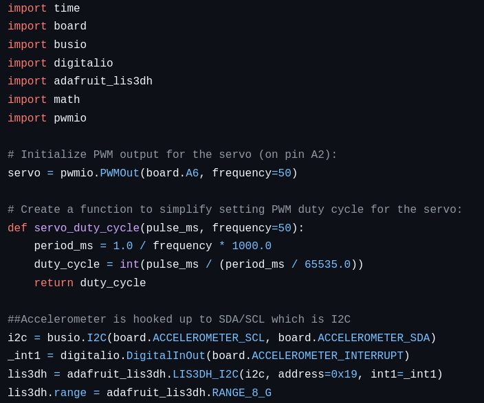
The first 22 lines here will hopefully seem familiar. Line 1-7 are import commands of all the various modules needed. Lines 10-13 create the definition that converts pulse width to duty cycle. Line 16 creates the servo and lines 19-22 create the accelerometer. Hopefully this is a good example of combining different codes together to get a more complex piece of software. Lines 24-45 include a very long while loop. I will try and go through each line. Line 26 grabs the accelerometer data on the CPX. Line 28 uses the x and z axis accelerometer data and converts the values to pitch angle using the atan2 function in the math module which was imported on line 4. Line 30 computes the elevator pitch angle and line 32 computes the servo deflection angle. Line 34-37 is a type of signal conditioner called a saturation filter. Basically, I don’t want the servo to break because I tried to make the servo rotate more than 180 degrees or less than 0 degrees. So I created two if statements that restrict the servo to be within these two values. If the servo angle is less than 0 as stated on line 34, the servo angle is set to 0 on line 35. If the servo angle is greater than 180 as stated in line 36 the servo angle is set to 180.
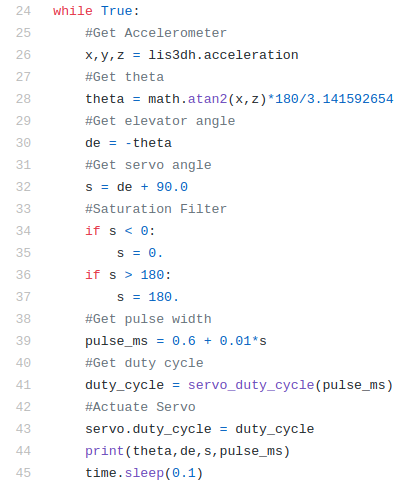
Line 39 uses the calibration equation from the previous experiment to convert servo angle to pulse width. You’ll need to replace these numbers with your servo since all servos are different. Line 41 uses the definition created on lines 10-13 to convert pulse width to duty cycle. Line 43 makes the servo move. Line 44 prints everything to Serial for debugging purposes and line 45 pauses the script for 0.1 seconds which helps with some twitchiness in the servo. When I did this I didn’t have to program a complementary filter so I guess the servo may have it’s own low pass filter. Either way this circuit is ready to be placed on an aircraft. Whether or not it is effective is a completely different story.
Subsection 19.3.2 Second Order Pitch Dynamics
We could take an entire aircraft design course or an undergraduate controls and systems dynamics course but to start let’s just simulate this control system and see how it does. First we need to write the dynamic equation for pitch of an aircraft. That is shown below.
\begin{equation}
\frac{J}{q_{\infty}S\bar{c}}\ddot{\theta} - \frac{\bar{c}}{2u_0}C_{mq}\dot{\theta} - C_{m\alpha}\theta = C_{m\delta_e}\delta_e + C_{m0}\tag{19.3.6}
\end{equation}
In the equation above \(J\) is the inertia of the aircraft, \(C_{m0},C_{mq},C_{m\alpha}\) and \(C_{m\delta_e}\) are non-dimensional coefficients, \(\bar{c}\) is the mean aerodynamic chord, \(u_0\) is the equilibrium velocity, \(\bar{c}\) is the mean aerodynamic chord, S is the planform area of the wing and \(q_{\infty}\) is the dynamic pressure. The dynamic pressure is given by the equation below
\begin{equation}
q_{\infty} = \frac{1}{2}\rho {u_0}^2\tag{19.3.7}
\end{equation}
where \(\rho\) is the air density. To simulate this system use the table below.
| \(C_{m\alpha}\) | -2.19 | \(C_{mq}\) | -24.45 | \(C_{m\delta_e}\) | -1.15 |
| \(\bar{c}\) | 0.2286 m | S | 0.34 \(m^2\) | J | 0.1232 \(kg-m^2\) |
| \(u_0\) | 15 m/s | \(\rho\) | 1.225 \(kg/m^3\) | \(C_{m0}\) | -0.076 |
Now that the dynamics are written, the second order equation can be integrated using a standard numerical tool. In this case it’s safe to assume the angular velocity is zero and the initial pitch angle is also zero. You can then use proportional control to command your pitch angle to whatever you want. Note that proportional control is not sufficient to stabilize your aircraft but I’ll leave that discussion to your controls professor.
Subsection 19.3.3 First Order Velocity Dynamics
In order to gain some practice with simulating dynamic systems it’s possible to approximate the velocity of an aircraft as a first order system. In order to accelerate a radio controlled aircraft, the motor must spin faster. It turns out that the PWM commands sent to servos to cause them to rotate back and forth is actually the same PWM signal used to control an Electronic Speed Controller (ESC) which controls a motor. So if you send around 1.1 ms to an ESC, the motor will be off and 1.9 ms will be full throttle. In this case we can make a simple equation that relates the throttle command to the velocity of the aircraft. The equation is shown below.
\begin{equation}
\dot{u} = \frac{1}{m}[C_{x\delta t} (\delta_t-\delta_0) - 0.5\rho u_0 S C_x u]\tag{19.3.8}
\end{equation}
where \(m=1.23 kg\text{,}\) \(u\) is the velocity of the aircraft, \(\delta_t\) is the throttle command in \(ms\text{,}\) and \(\delta_0=1.1 ms\) is the nominal PWM pulse to an ESC. The coefficients \(C_{x\delta t}=13.78 \frac{N}{ms}\) and \(C_x=0.017\) are coefficients that relate throttle to acceleration and velocity to drag respectively. The rest of the variables are explained above in the second order system. For this simulation you can assume that proportional control works just fine and thus
\begin{equation}
\delta_t = k_p(u_c-u)\tag{19.3.9}
\end{equation}
where \(u_c\) is the commanded velocity and \(k_p\) is the proportional gain.
