The light sensor on the CPX is just a simple photocell wired in series with a resistor. A photocell (or Light Dependent Resistor, LDR) is a sensor whose resistance changes significantly based on the intensity of light falling on its sensitive surface. In dimmer light, its resistance is high, and in brighter light, its resistance is low. By integrating it into a simple voltage divider circuit, Adafruit makes it possible to read the voltage across the photocell and correlate that to light level. There is a relevant Adafruit Tutorial on Photocells and the code required to measure the voltage if you’d like to read more about it[32].
The GND leg of the photocell is connected to pin A8. You can check the pin by looking at the graphic of an eye on the CPX and taking a look at the digital pin next to it. Since this circuit is connected to a voltage divider, the equations below can be used to relate the resistance in the photocell to the voltage being read by the ADC.
In this case \(V_{out}\) is 3.3V and \(R_{series}=10000 \Omega\) is a resistor value chosen by Adafruit. So, if you measure \(V_{photocell}\) using the ADC on the CPX/CPB you’ll be able to solve for the resistance in the photocell \(R_{photocell}\text{.}\) The resistance can then be used to determine the Lux value. Some sources suggest that Lux is a power law given by the equation below [48][61].
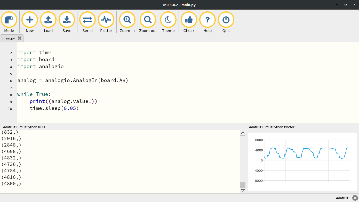
where \(R_{photocell}\) is the resistance of the photocell in Ohms. We’ve already learned how to access analog pins (See Chapter 13) in a previous lab so just use the code from that lab and change the pin to A8[33]. Here’s what my code looks like when I change the pin to A8. I also brought the Plotter up and moved my finger in front of the light to make sure the light was working. Verify that your CPX responds the same way before moving on.
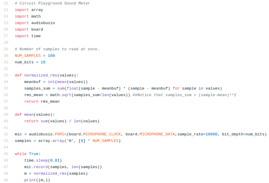
The sound sensor uses the audiobusio library and creates a mic object using the (Pulse Density Modulation) PDM library. You have to set the sample rate and the number of bits to use to capture the data. We’re going to set the bits to 16 to utilize the whole spectrum and then set the sample rate to 16 kHz. It’s not quite 44.1 kHz like most modern microphones but it will do. After creating the mic object we have to compute some root mean squared values and thus two functions are defined before the while true loop in the code. The code itself is shown below. The code starts on line 22 because the first 22 lines are copyright from Dan Halbert, Kattni Rembor, and Tony DiCola from Adafruit Industries[32]. I have edited the code a bit to fit my needs and uploaded my version to Github[33]. In the code line 23-27 import standard modules as well as some new ones. The array module is used to create array like matrices. The math module is used to compute functions like cos, sin, and sqrt. Then of course the audiobusio module is used to create the mic object on line 42. Notice the two functions defined on 33 and 39 which create a function for computing the mean and for computing the normalized root mean square value of the data stream. Basically what’s going to happen is we’re going to record 160 samples as defined on line 160. So on line 43 we create a hexadecimal array (hexademical: base 16 hence the num_bits set to 16 on line 31) with 160 zeros. In the while true loop we’re going to sleep for 0.01 seconds and then record some samples. Since we’re sampling at 16 kHz the time it takes to record 160 samples is 160/16000 = 16/1600 = 1/100 = 0.01 seconds. Since we’re taking 160 samples we need to compute some sort of average which is why the normalized root mean square value is computed on line 48.
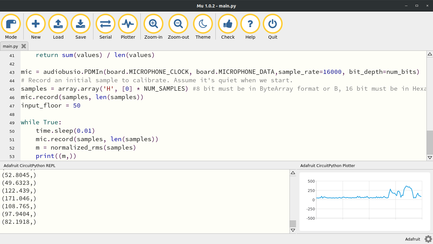
When I run this code and talk normally into the microphone, I get this output in the Plotter. You’ll notice that the data is pretty noisy in the beginning but then there are noticeable humps in the data. This is me saying something random into the microphone at normal volume. It’s possible we could increase the number of samples we take each loop by editing line 30 but that would slow down our code. So there’s a tradeoff between filtering here and speed. That’s something will investigate in some later labs.
The temperature sensor is actually a thermistor[63]. A thermistor is basically a “thermometer resistor” which means the resistance depends on temperature. Since this thermistor on the CPX/CPB is connected to an analog pin, you can read the analog signal coming from the thermistor just by reading the analog signal from pin A9. If you look for the thermometer symbol on the CPX you’ll see pin A9. Therefore, it is possible to just use the analogio library and just read in the analog voltage but in order to convert to celsius and then fahrenheit you need to use some heat transfer equations to convert the analog signal to celsius.
In this case, the thermistor is wired in a voltage divider circuit in series with a \(10000~\Omega\) resistor. For this circuit though, it turns out that the thermistor is actually wired to the high side of the voltage divider. That means when you measure pin A9 you’re actually measuring the voltage across the series resistor rather than the thermistor. This means that the voltage across the series resistor must be inverted to compute the resistance across the thermistor. This is done using the equation below similar to the equation used for the photocell.
Where \(V_{out}=3.3V\) and \(R_{series}=10000~\Omega\text{.}\) The equation above can be inverted to obtain the resistance in the thermistor . This means that the digital output from the analog to digital converter can be converted to voltage and then to resistance as has been done for various ADC labs in this textbook. Remember that the ADC on boad the CPX/CPB is actually measuring the digital output \(D_o\text{.}\) This can be converted to measured voltage as shown in the equation below
So the process is to first read the digital output from the ADC, convert that to voltage, then use the voltage to compute the resistance in the thermistor and finally use the resistance to compute the temperature in Kelvin. In order to convert measured voltage to resistance, we can rearrange the equations above to get the equation below
Note that \(V_{out}/V_{measured}=65535/D_o\text{.}\) Once you have the resistance from the thermistor, you can use a modified version of the Stein-Hart[64][65] to convert the resistance to temperature in Celsius.
where \(\beta=3950\) is a heat transfer coefficient specific to the bulk semiconductor material over a given temperature range of interest and \(T_0=298.15K\) is the nominal temperature of the semiconductor in Kelvin. Note that in the equation above, the output is in Kelvin.
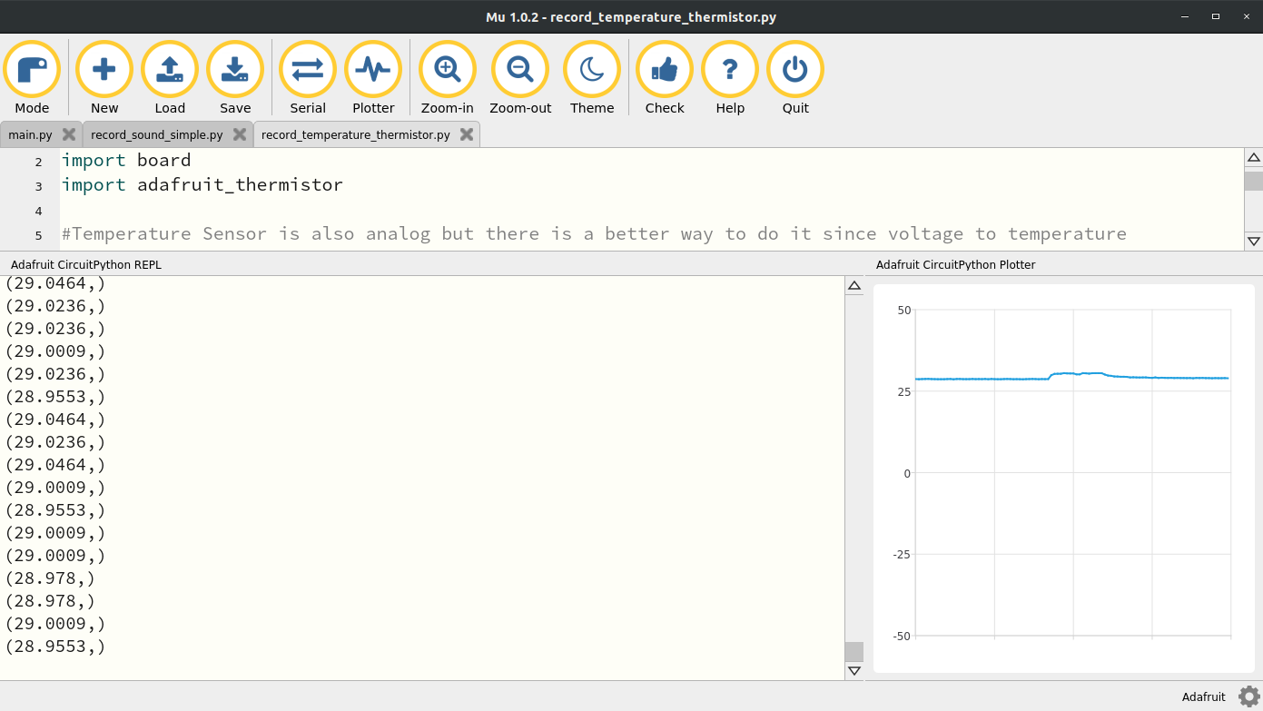
If this all seems complex, the folks at Adafruit have done it again with an adafruit_thermistor module. If you head over to their github on this module you’ll see the relevant conversion under the definition temperature which at the time of this writing is on line 127[33]. The Adafruit Learn system also does a bit of work to explain the conversion from voltage to temperature[32] but understand that the tutorial on that page assumes that the thermistor is on the low (grounded) side and thus the voltage divider equation is different. If you look at the adafruit_thermistor module you’ll see that there is a self.high_side boolean that changes between either a thermistor on the high side or the low side. In this case, for the built-in A9 thermistor the thermistor is on the high side. Given all this complexity, we will just appreciate the simplicity of the code below which uses the adafruit_thermistor module. I’ve also created a simple version of the code to read the analog value of the thermistor and posted it on my Github[33]. Note the code below is from a much earlier and simpler version of my code which only reads the temperature in Celsius. The code on my Github has more functionality such as printing the raw ADC value and the voltage.
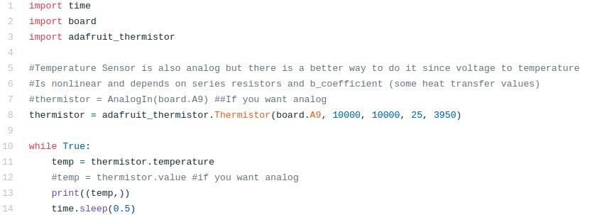
For the code above, lines 1-3 import the relevant modules and then line 8 create the thermistor object. You’ll notice the input arguments are the pin which is A9 as well as the resistor values which are in series with the thermistor. These resistors are soldered to the PCB so they are fixed at \(10 k\Omega\text{.}\) The 25 is for the nominal resistance temperature in celsius of the thermistor and 3950 is the b coefficient which is a heat transfer property. Running this code and then placing my finger on the A9 symbol causes the temperature to rise just a bit. You’ll notice the temperature rise quite quickly when I place my finger on the sensor but when I remove the sensor it takes some time before the sensor cools off. This has to do with the dynamic response of the sensor. We’ll discuss this in some future labs on dynamic measurements. For now you can move on to the accelerometer.
The accelerometer is a 3-axis sensor. As such, it is going to spit out not just 1 value but 3 values. Accelerations in x,y and z or North, East, Down or Forward, Side to Side, Up and Down. Since it’s reading 3 values we can’t just read 3 analog signals (we can but the accelerometer chip design didn’t want to do that) so instead we’re going to use the I2C (I like "Indigo" and 2C like "Squared C". So "I Squared C". Not "12C" or "one two C". It’s "I squared C") functionality. I2C is a type of serial communication that allows computers to send strings rather than numbers. I2C is beyond the scope of this course but just know it’s a type of serial communication that uses hexadecimal addresses. It’s a much more complex form of communication but since it’s a standard form of communication, we can just use the busio module which contains the I2C function.
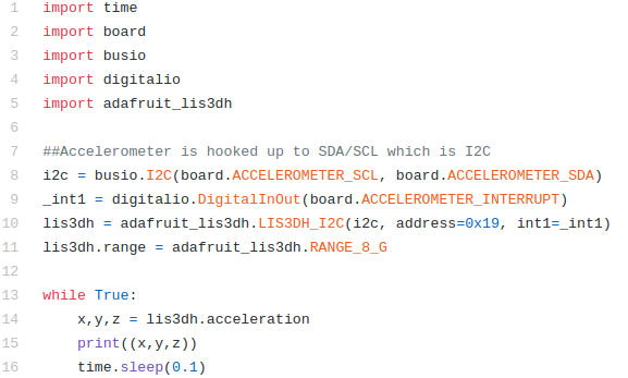
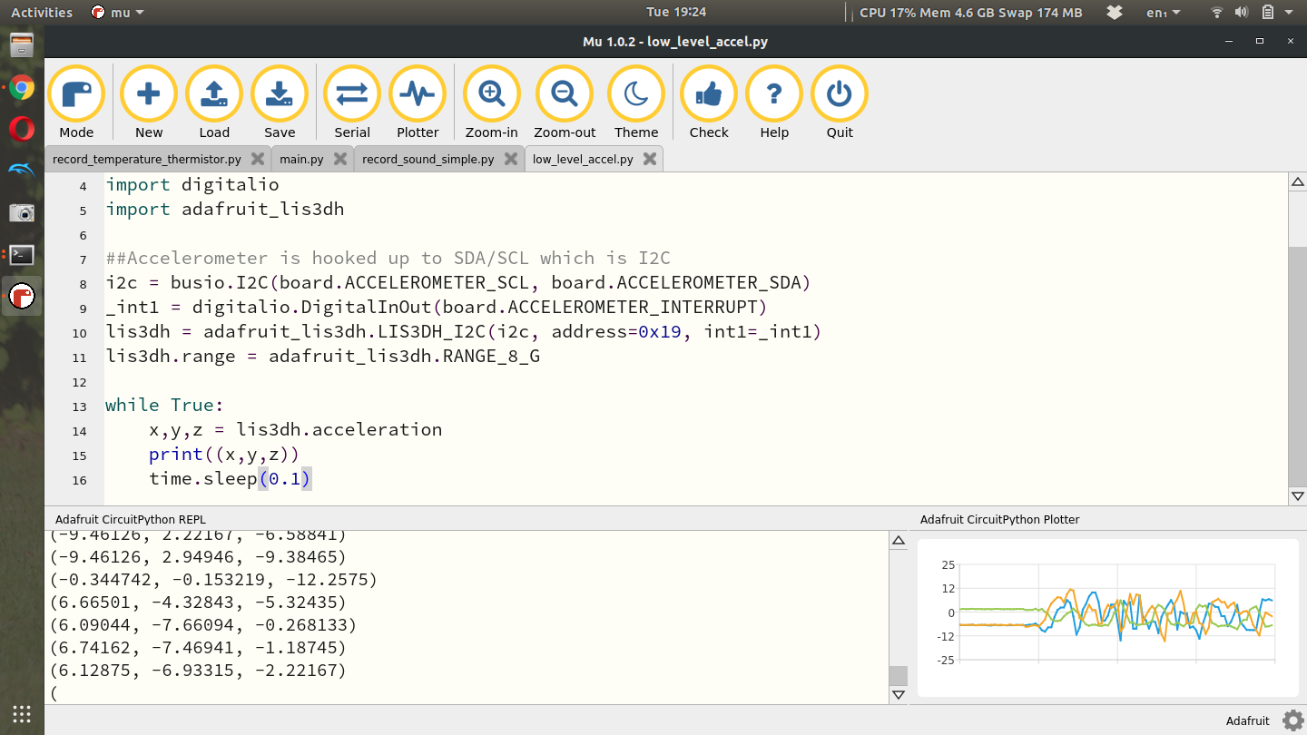
In this code we see alot more imports than normal. In addition to the standard time, board and digitalio modules we need the busio module and the adafruit_lis3dh. You might think that LIS3DH is a very weird name for an accelerometer but it’s actually the name of the chip on your CPX. The chip itself is very standard and is well documented on multiple websites. Here’s one from ST[66]. You can also buy the chip on a breakout board from Adafruit and then of course the Adafruit Learn site has plenty of tutorials on reading Accelerometer data in CircuitPython[32][34]. As always I’ve learned what I can from the relevant tutorials and created my own simple version to read the accelerometer data and posted it to Github[33]. I digress, lines 8-11 of the code do alot. It first uses the SCL and SDA pins to set up an I2C object which establishes serial communication to the accelerometer. Line 9 creates an interrupt which is beyond the scope of this course. Finally, line 10 creates the actual accelerometer object by sending it the I2C pins, the hexadecimal address in the I2C protocol and finally the interrupt pin. Line 11 then sets the range. Line 14 in the while loop is where the x,y and z values of the accelerometer are read and then promptly printed to Serial on line 15. If I run this code and shake the sensor a bit I can get all the values to vary. If you put the CPX on a flat surface, the Z axis will measure something close to 9.81. The units of the accelerometer are clearly in \(m/s^2\text{.}\)
Figure15.1.7.Serial monitor and Plotter open in Mu showing accelerometer output in \(m/s^2\)
Note that the accelerometer can be used to obtain pitch and roll angles in benign environments. This is done via trigonometry. You’ll notice that when you point the CPX directly at you with the cable pointing up the x axis reads around 0 and the y axis reads around gravity. If you then rotate the sensor so that the cable is coming out of the left side of the CPX, the x axis is reading about gravity while the y axis is zero. Similarly, rotating the CPX in the X/Z plane can be done by rotating the USB cable where it plugs into the CPX. In this case we can ignore the Y axis data. If you print the raw accelerometer data, you’ll notice that when you place the CPX directly onto a flat surface, the x and y axes read a value around 0, while the z axis reads around gravity (9.81\(m/s^2\)). If you then rotate the sensor clockwise 90 degrees, the x axis is reading about gravity while the z axis is now zero. This means we can form two triangles (one for the X/Z plane and another for the Y/Z plane) and get the angles of the CPX/CPB using the equations below.
In the equations above, \(a\) is the accelerations along all 3 axes. Shorthand is used for \(cos(\eta)=c_{\eta}\) and \(sin(\eta)=s_{\eta}\text{.}\) The \(\bar{\eta}\) notation is used to indicate a normalization of the vector. That is \(\bar{\eta} = \eta/||\eta||\) where \(||\eta||\) is the norm of a 3 dimensional vector \(||\eta||=\sqrt{\eta_x^2+\eta_y^2+\eta_z^2}\text{.}\) The derivation for these angles from accelerometers is quite involved and requires the knowledge of rotation matrices. That derivation is in another textbook called Aerospace Mechanics[33].