Section 19.2 Servo Calibration
If you notice, sending a pulse signal in microseconds moved the servo to a specific angle. Thing is I would like to be able to move the servo to a specific angle rather than having to just guess and check like we did in the last lab. So what we’re going to do is start at the minimum pulse signal you computed in the last project and then change the servo pulse in equal increments until we reach the maximum servo pulse signal. When I did this lab I found that 0.6 ms was just about the smallest I could get the servo to move. We’re going to call this 0 degrees. My maximum pulse signal ended up being about 2.4 ms. So I want you to test 10 different points between your specific maximum and minimum value which will hopefully be different for all of you. Everytime you test a pulse I want to measure the angle the servo makes with the minimum value being 0 degrees. Create a table of data with two columns. In the first column put pulse in milliseconds and in the second column put angle of servo in degrees. Use a protractor to measure the angle. If you don’t have a protractor you can actually build one or just pull up a protractor on your computer screen and use that. I did this project with just 3 data points and here are my data points. Again you need to have around 10 data points.
| Pulse (ms) | Angle (Degrees) |
| 0.6 | 0 |
| 1.5 | 90 |
| 2.4 | 180 |
Take your table of data and put it into a spreadsheet and save the data as a CSV or simply put your data into a text file. Since I only had 3 data points I just put them into a text file. Plot the data on your desktop computer with servo angle on the x-axis and duty cycle on the y axis. Using the data, determine if the data set is linear, quadratic or cubic. Fit a trend line to the data and plot your trend line on top of the data. I made a helpful python script with some fictitious data on Github that fits the data with linear and quadratic fits[33]. Here is my data plotted alongside the trendline in Python. I sort of made up the data and made it perfect on purpose so my trendline is perfect. Yours will not be so perfect.
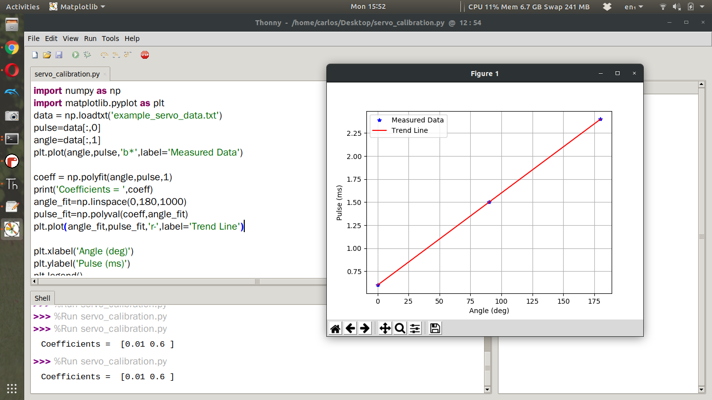
You’ll notice that I first import the data from the text file using the np.loadtxt function and then I use the polyfit and polyval functions to create the trendline. The polyfit function requires you to give it the X and Y axes and the order of the trendline which since the trend line is linear I sent it a 1 but you could easily do 2 for quadratic or 3 for cubic. I then print the coefficients which are [0.01 0.6]. This means my trend line looks like this.
\begin{equation}
Pulse = 0.6 + 0.01*Angle\tag{19.2.1}
\end{equation}
Where Pulse is in ms and Angle is in degrees. Now you have an equation where you can use angle in degrees to compute the pulse in milliseconds. In the code I’ve posted I then use np.linspace to create 1000 data points from 0 to 180 degrees and then use the polyval function to compute the pulse for all 1000 angles I created using the linspace command. I finally plot the trend line in red and use the remaining part of the script to create labels and legends. Once you have this plot write down your coefficients and create an equation like I did above. Again your numbers won’t be so neat. Once you have this equation, return to Mu and create a function using the def keyword that takes in an angle as an input and then returns a pulse signal in milli seconds. It will look sometime like this
def angle2pulse(angle):
        return 0.6 + 0.01*angle
Note: Functions in python must be after all your imports but before your while loop. If you put this function inside your while loop the code will not work. Using that equation, modify your servo.py script to have the servo move through the following angles, 0, 45,90,135 (your servo may not travel to 180 degrees). Verify that your equation is working correctly by placing your protractor below the servo. Much of the code required for this project is not included because it is left as an exercise for the student.
